The white furnace test

The white furnace test is one of my favourite rendering debug tools. But before it was so, it was rather mysterious and abstract to me. Why would a publication proudly show what seemed like empty renders? What does it mean, and why would they care?

Slide from the presentation Revisiting Physically Based Shading at Imageworks, in which a white furnace test of the diffuse term is shown.
What’s up with the empty grey rectangle? The fact that looks empty is the point.
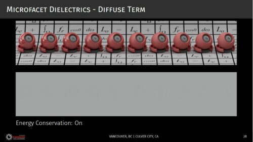
Revisiting Physically Based Shading at Imageworks, presented at the SIGGRAPH 2017 course: Physically Based Shading in Theory and Practice.

The idea is the following: if you have a 100% reflective object that is lit by a uniform environment, it becomes indistinguishable from the environment. It doesn’t matter if the object is matte or mirror like, or anything in between: it just “disappears”.

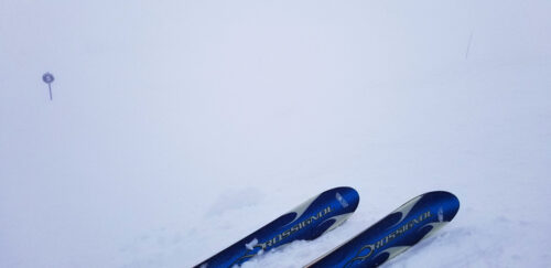
Accepting this idea took me a while, but there is a real-life situation in which you can experience this effect. Fresh snow can have an albedo as high as 90% to 98%, i.e. nearly perfect white. Associated with overcast weather or fog, it can sometimes appear featureless and become completely indistinguishable from the sky, to the point you’re left with skiing by feel because you can’t even tell the slope two steps in front of you. Everything is just a uniform white in all directions: the whiteout.

Photo taken on a ski track. The ground appears almost uniformly white.
Last time I visited a white furnace test. Note how the snow surface slope and details are almost invisible, and the sign in the background seems to be floating in the air.

With the knowledge that a 100% reflective object is supposed to look invisible when uniformly lit, verifying that it does is a good sanity test for a physically based renderer, and the reason why you sometimes see those curious illustrations in publications. It’s showing that the math checks out.

Those tests are usually intended to verify that a BRDF is energy preserving: making sure that it is not losing or adding energy. A typical topic for example is making sure materials don’t look darker as roughness increases and inter-reflections become too significant to be neglected. Missing energy is not the only concern though, and a grey environment (as opposed to a white one) is convenient as any excess of reflected energy will appear brighter than it.

Demonstration of the white furnace test on ShaderToy, or an expensive way to render an empty image. Press the play button to see the scene revealed.

But verifying the energy conservation of a BRDF is just one of the cases where the white furnace test is useful. Since a Lambertian BRDF with an albedo of 100% is perfectly energy preserving and completely trivial to implement, the white furnace test with such a white Lambert material can be used to reveal bugs in the renderer implementation itself.

There are so many aspects of the implementation that can go wrong: the sampling distribution, the proper weighting of the samples, a mistake in the PDF, a pi or a 2 factor forgotten somewhere… Those errors tend to be subtle and can result in a render that still looks reasonable. Nothing looks more like a correct shading than a slightly incorrect one.

So when I’m either writing a path tracer or one of its variants, or generating a pre-convolved environment map, or trying different sampling distributions, my first sanity check is to make sure it passes the white furnace test with a pure white Lambertian BRDF. Once that is done (and as writing the demonstration shader above showed me once again, that can take a few iterations), I can have confidence in my implementation and test the BRDF themselves.

Take away: the white furnace test is a very useful debugging tool to validate both the integration part and the BRDF part of your rendering.

Update: A comment on Hacker News mentioned that it would be useful to see an example of what failing the test looks like. So I’ve added a macro SIMULATE_INCORRECT_INTEGRATION in the shader above, to introduce a “bug”, the kind like forgetting that the integration over an hemisphere amounts to 2Pi or forgetting to take the sampling distribution into account for example. When the “bug” is active, the sphere becomes visible because it doesn’t reflect the correct amount of energy.

A list of path tracing shaders

I have gathered a list of path tracing shaders on ShaderToy.

Path tracing is a surprisingly simple technique to render realistic images. This would be my definition if you are unfamiliar with the term. But if you already have experience with various ray tracing techniques, I would probably say that path tracing is a remarkably elegant solution to the rendering equation. You can implement a toy path tracer in a weekend or, if you’ve already done it a few times before, within 25 minutes.

Recently I was documenting myself on path tracing, and some of the techniques that can be used, like next event estimation, bidirectional path tracing, Russian roulette, etc. This is a case where ShaderToy can be an invaluable source of examples and information, and so I was browsing path tracing shaders there. As the number of open tabs was starting to get impractical, I decided to use the “playlist” feature of ShaderToy to bookmark them all.

You can find the list here: Path tracing, on ShaderToy.

The examples of path tracers listed include very naive implementations, hacky ones, rendering features like advanced BRDF, volumetric lighting or spectral rendering, or various noise reduction techniques such as next event estimation, bidirectional path tracing, multiple importance sampling, accumulation over frames with temporal reprojection, screen space blue noise, or convolutional neural network based denoising.

Some of those shaders are meant to be artworks, but even the technical experimentation ones look nice, because the global illumination inherent to path tracing tends to generate images that are pretty.

Screenshot of the list on ShaderToy, with various kinds of path tracers visible.

Practical Pigment Mixing for Digital Painting

About a year ago at SIGGRAPH Asia 2021 (which took place as a hybrid conference both online and on site at the Tokyo International Forum) one of the technical papers that caught my attention was the publication by Šárka Sochorová and Ondřej Jamriška on color mixing.

Color mixing in most digital painting tools is infamously unsatisfying, often limited to a linear interpolation in RBG space, resulting in unpleasing gradients very different from what one would expect. Ten years ago I mentioned this article that presented the color mixing of the application Paper, which tried to solve this very problem.

This time, the core idea is to model colors as pigments: estimate the pigment concentration based on the color, so in a way, move from RGB space to “pigment space”, and interpolate the pigment concentration, before converting back to RGB space.

The paper uses the Kubelka-Munk model for estimating colors from pigment concentration. The problem however is to find a transformation between the two spaces. A first assumption is made on the available pigments: essentially restricting them to CMYK. Then two problems are addressed: RGB colors that cannot be represented with those pigments, and likewise pigment colors that cannot be represented in RGB.
The paper proposes a remapping that enables a transform and its inverse, thus allowing to move from RGB space to pigment space, interpolate in pigment space, and move back to RGB space.

You could argue this is therefore a physically based diffuse color mixing.

Finally, the implementation of the proposed model, Mixbox, is available under a CC BY-NC license:
https://github.com/scrtwpns/mixbox

Two Minute Papers did a video on this paper as well:

https://youtube.com/watch?v=b2D_5G_npVI

Overview of global illumination in Tomasz’s kajiya renderer

Soon after showcasing his recent rendering results which left industry veterans impressed and causing many of us to start documenting ourselves about ReSTIR, professional madman Tomasz Stachowiak showed a new demonstration of the global illumination capabilities of his pet project.

This is what some people manage to do with just seven months of tinkering…

But more importantly, he took the time to describe the techniques used to get such results. The writing is fairly high level, and assumes the reader to be familiar with several advanced topics, but it comes with clear illustrations at least for some parts. It also mentions the various ways in which ReSTIR is leveraged to support the techniques used. Finally, it doesn’t try to hide the parts where the techniques fall short, quite the opposite.

The article: Global Illumination overview.

In very brief, the rendering combines a geometry pass, from which a ReSTIR pass is done to compute the first bounce rays, in combination with a sparse voxel grid based irradiance cache for the rest of the light paths, which also relies on ReSTIR, and a few clever tricks to handle various corner cases, as well as denoising and temporal anti-aliasing to smooth things out.

Reading list on ReSTIR

Recently a short video from dark magic programmer Tomasz Stachowiak made the rounds in the graphics programming community, at the sound of jaws hitting the floor in its wake. It shows his recent progress on in his renderer pet project: beautiful real-time global illumination with fast convergence and barely any noise, in a static environment with dynamic lighting.

In a Twitter thread where he discussed some details, one keyword in particular caught my attention: ReSTIR.

ReSTIR stands for “Reservoir-based Spatio-Temporal Importance Resampling” and is a sampling technique published at SIGGRAPH 2020 and getting refined since.

The original publication

Spatiotemporal reservoir resampling for real-time ray tracing with dynamic direct lighting
The publication page includes the recording of the SIGGRAPH presentation, with a well articulated explanation of the technique by main author Benedikt Bitterli.
(same publication hosted on the NVidia website).

Explanations of ReSTIR

Improvements over the original publication

After the initial publication, NVidia published a refined version producing images with less noise at a lower cost, which they call “RTXDI” (for RTX Direct Illumination).

Other limitations

When discussing on Twitter some of the limitations of ReSTIR, Chris Wyman made the following remarks:

To be clear, right now, ReSTIR is a box of razor blades without handles (or a box of unlabeled knobs). It’s extremely powerful, but you have to know what you’re doing. It is not intuitive, if your existing perspective is traditional Monte Carlo (or real-time) sampling techniques.

People sometimes think SIGGRAPH paper = solved. Nope. We’ve learned a lot since the first paper, and our direct lighting is a lot more stable with that knowledge. We’re still learning how to do it well on full-length paths.

And there’s a bunch of edge cases, even in direct lighting, that we know how to solve but haven’t had time to write them up, polish, and demo.

We haven’t actually tried to solve the extra noise at disocclusions in (what I think of as) a very principled way. Right now a world-space structure is probably the best way. I’m pretty sure it can be done without a (formal) world-space structure, just “more ReSTIR.”

Building an artificial window

Several years ago, I mentioned the Italian company CoeLux, which specializes in making artificial windows: light fixtures that look like sunlight in a clear blue sky.

The price of their products is apparently in the range of several tens of thousands of dollars (I’ve heard prices like $20k to 50k), which makes it out of reach for most individuals. Not many details about their invention are available either (from the promotion material: LED powered, several hundred watts of electrical power, a solid diffuse material, and a thickness around 1 meter), and I was left wondering what was the secret sauce to their intriguing technology.

The window in this photo is in fact an electrical light fixture.

The YouTube channel DIY Perks has been working on day light projects for a while now, improving at each iteration. Yesterday they published a video explaining how to build a light that seems to give very similar results as CoeLux’s product, from some basic materials that are fairly simple to find. Since their solution takes roughly the same volume, it’s tempting to think it uses the same technique

It’s extremely satisfying to finally see how this works and, despite the practical aspects, quite tempting to try if only to see how it looks in real life.

Intersection of a ray and a plane

I previously showed the derivation of how to determine the intersection of a plane and a cone. At the time I had to solve that equation, so after doing so I decided to publish it for anyone to use. Given the positive feedback, it seems this was useful, so I might as well continue with a few more.

Here is probably the most basic intersection: a ray and a plane. Solving it is straightforward, which I hope can be seen below. Like last time, I am using vector notation.

  1. We define a ray with its origin $O$ and its direction as a unit vector $\hat{D}$.
    Any point $X$ on the ray at a signed distance $t$ from the origin of the ray verifies: $\vec{X} = \vec{O} + t\vec{D}$.
    When $t$ is positive $X$ is in the direction of the ray, and when $t$ is negative $X$ is in the opposite direction.
  2. We define a plane with a point $S$ on that plane and the normal unit vector $\hat{N}$, perpendicular to the plane.
    The distance between any point $X$ and the plane is $d = \lvert (\vec{X} – \vec{S}) \cdot \vec{N} \rvert$. If this equality is not obvious for you, you can think of it as the distance between $X$ and $S$ along the $\vec{N}$ direction. When $d=0$, it means $X$ is on the plane itself.
  3. We define $P$ the intersection or the ray and the plane, and which we are interested in finding.

Since $P$ is both on the ray and on the plane, we can write: $$ \left\{ \begin{array}{l} \vec{P}=\vec{O} + t\vec{D} \\ \lvert (\vec{P} – \vec{S}) \cdot \vec{N} \rvert = 0 \end{array} \right. $$ Because the distance $d$ from the plane is $0$, the absolute value is irrelevant here. We can just write: $$ \left\{ \begin{array}{l} \vec{P}=\vec{O} + t\vec{D} \\
(\vec{P} – \vec{S}) \cdot \vec{N} = 0 \end{array} \right. $$ All we have to do is replace $P$ with $\vec{O} + t\vec{D}$ in the second equation, and reorder the terms to get $t$ on one side.
$$ (\vec{O} + t\vec{D} – \vec{S}) \cdot \vec{N} = 0 $$ $$ \vec{O} \cdot \vec{N} + t\vec{D} \cdot \vec{N} – \vec{S} \cdot \vec{N} = 0 $$ $$ t\vec{D} \cdot \vec{N} = \vec{S} \cdot \vec{N} – \vec{O} \cdot \vec{N} $$ $$ t = \frac{(\vec{S} – \vec{O}) \cdot \vec{N}}{ \vec{D} \cdot \vec{N} } $$

A question to ask ourselves is: what about the division by $0$? Looking at the diagram, we can see that $\vec{D} \cdot \vec{N} = 0$ means the ray is parallel to the plane, and there is no solution unless $O$ is already on the plane. Otherwise, the ray intersects the plane for the value of $t$ written above. That’s it, we’re done.

Note: There are several, equivalent, ways of representing a plane. If your plane is not defined by a point $S$ and a normal vector $\hat{N}$, but rather with a distance to the origin $s$ and a normal vector $\hat{N}$, you can notice that $s = \vec{S} \cdot \vec{N}$ and simplify the result above, which becomes: $$ t = \frac{s – \vec{O} \cdot \vec{N}}{ \vec{D} \cdot \vec{N} } $$


Signed distance to a plane

For the sake of simplicity, in the above we defined the distance to the plane as an absolute value. It is possible however to define it as a signed value: $d = (\vec{X} – \vec{S}) \cdot \vec{N}$. In this case $d>0$ means $X$ is somewhere on the side of the plane pointed by $\vec{N}$, while $d<0$ means $X$ is on the opposite side of the plane.

Distances that can be negative are called signed distances, and they are a foundation of Signed Distance Fields (SDF).