Some time ago I needed to solve analytically the intersection of a ray and a cone. I was surprised to see that there are not that many resources available; there are some, but not nearly as many as on the intersection of a ray and a sphere for example. Add to it that they all use their own notation and that I lack math exercise, after a bit of browsing I decided I needed to write a proof by myself to get a good grasp of the result.
So here goes, the solution to the intersection of a ray and a cone, in vector notation.
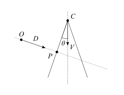
- We define a ray with its origin $O$ and its direction as a unit vector $\hat{D}$.
Any point $X$ on the ray at a signed distance $t$ from the origin of the ray verifies: $\vec{X} = \vec{O} + t\vec{D}$.
When $t$ is positive $X$ is in the direction of the ray, and when $t$ is negative $X$ is in the opposite direction.
- We define a cone with its tip $C$, its axis as a unit vector $\hat{V}$ in the direction of increasing radius, and $\theta$ the half angle between the axis and the surface.
Any point $X$ on the cone verifies: $(\vec{X} – \vec{C}) \cdot \vec{V} = \lVert \vec{X} – \vec{C} \rVert \cos\theta$
- Finally we define $P$ the intersection or the ray and the cone, and which we are interested in finding.
$P$ verifies both equations, so we can write:
$$
\left\{
\begin{array}{l}
\vec{P}=\vec{O} + t\vec{D} \\
\frac{ \vec{P} – \vec{C} }{\lVert \vec{P} – \vec{C} \rVert} \vec{V} = \cos\theta
\end{array}
\right.
$$
We can multiply the second equation by itself to work with it, then reorder things a bit.
$$
\left\{
\begin{array}{l}
\vec{P}=\vec{O} + t\vec{D} \\
\frac{ ((\vec{P} – \vec{C}) \cdot \vec{V})^2 }{ (\vec{P} – \vec{C}) \cdot (\vec{P} – \vec{C}) } = \cos^2\theta
\end{array}
\right.
$$
$$
\left\{
\begin{array}{l}
\vec{P}=\vec{O} + t\vec{D} \\
((\vec{P} – \vec{C}) \cdot \vec{V})^2 – (\vec{P} – \vec{C}) \cdot (\vec{P} – \vec{C}) \cos^2\theta = 0
\end{array}
\right.
$$
Remember the mouthful earlier about $\hat{V}$ being in the direction of increasing radius? By elevating $\cos\theta$ to square, we’re making negative values of $\cos$ positive: values of $\theta$ beyond 90° become indistinguishable from values below 90°. This has the side effect of turning it into the equation of not one, but two cones sharing the same axis, tip and angle, but in opposite directions. We’ll fix that later.
We replace $\vec{P}$ with $\vec{O} + t\vec{D}$ and work the equation until we get a good old quadratic function that we can solve.
$$
\require{cancel}
((\vec{O} + t\vec{D} – \vec{C})\cdot\vec{V})^2 – (\vec{O} + t\vec{D} – \vec{C}) \cdot (\vec{O} + t\vec{D} – \vec{C}) \cos^2\theta = 0
$$
$$
((t\vec{D} + \vec{CO})\cdot\vec{V})^2 – (t\vec{D} + \vec{CO}) \cdot (t\vec{D} + \vec{CO}) \cos^2\theta = 0
$$
$$
(t\vec{D}\cdot\vec{V} + \vec{CO}\cdot\vec{V})^2 – (t^2\cancel{\vec{D}\cdot\vec{D}} + 2t\vec{D}\cdot\vec{CO} + \vec{CO}\cdot\vec{CO}) \cos^2\theta = 0
$$
$$
(t^2(\vec{D}\cdot\vec{V})^2 + 2t(\vec{D}\cdot\vec{V})(\vec{CO}\cdot\vec{V}) + (\vec{CO}\cdot\vec{V})^2) – (t^2 + 2t\vec{D}\cdot\vec{CO} + \vec{CO}\cdot\vec{CO}) \cos^2\theta = 0
$$
$$
t^2(\vec{D}\cdot\vec{V})^2
+ 2t(\vec{D}\cdot\vec{V})(\vec{CO}\cdot\vec{V})
+ (\vec{CO}\cdot\vec{V})^2
– t^2\cos^2\theta
– 2t\vec{D}\cdot\vec{CO}\cos^2\theta
– \vec{CO}\cdot\vec{CO}\cos^2\theta
= 0
$$
Reorder a bit:
$$
t^2((\vec{D}\cdot\vec{V})^2 – \cos^2\theta)
+ 2t((\vec{D}\cdot\vec{V})(\vec{CO}\cdot\vec{V}) – \vec{D}\cdot\vec{CO}\cos^2\theta)
+ (\vec{CO}\cdot\vec{V})^2 – \vec{CO}\cdot\vec{CO}\cos^2\theta
= 0
$$
There we go, we have our $at^2 + bt + c = 0$ equation, with:
$$
\left\{
\begin{array}{l}
a = (\vec{D}\cdot\vec{V})^2 – \cos^2\theta \\
b = 2\Big((\vec{D}\cdot\vec{V})(\vec{CO}\cdot\vec{V}) – \vec{D}\cdot\vec{CO}\cos^2\theta\Big) \\
c = (\vec{CO}\cdot\vec{V})^2 – \vec{CO}\cdot\vec{CO}\cos^2\theta
\end{array}
\right.
$$
From there, you know the drill: calculate the determinant $\Delta = b^2 – 4ac$ then depending on its value:
- If $\Delta < 0$, the ray is not intersecting the cone.
- If $\Delta = 0$, the ray is intersecting the cone once at $t = \frac{-b}{2a}$.
- If $\Delta > 0$, the ray is intersecting the cone twice, at $t_1 = \frac{-b – \sqrt{\Delta}}{2a}$ and $t_2 = \frac{-b + \sqrt{\Delta}}{2a}$.
But wait! We don’t have one cone but two, so we have to reject solutions that intersect with the shadow cone. $P$ must still verify $\frac{ \vec{P} – \vec{C} }{\lVert \vec{P} – \vec{C} \rVert} \vec{V} = \cos\theta$, or simply, if $\theta < 90°$: $(\vec{P} – \vec{C})\cdot\vec{V} > 0$.
Note that there is also the corner case of the ray tangent to the cone and having an infinity of solutions to consider. I’ve completely swept it under the rug since it doesn’t matter in the context I was, but if it does to you, you’ve been warned about it. Also remember to check the sign of $t$ to know whether $P$ is in the direction of the ray. You may need to determine which of $t_1$ or $t_2$ you want to use, which depends on your use case. For example is your ray origin inside or outside of the cone?
Now for a little sanity test, let’s consider the corner case $C=O$, where the ray origin is the tip of the cone (thanks Rubix for the suggestion!). We have $b=0$ and $c=0$ thus $\Delta=0$ and $t=\frac{-b}{2a}=0$ which is the expected result.
I also tried the cases $\theta=0$ and $\theta=\pi/2$, but expanding $\Delta$ proved too tedious to proceed to the end. So this is left as an exercise, as they say. :)
Finally, to demonstrate that the result is indeed correct, here is a glorious ray traced cone scene on ShaderToy:
I hope this can prove useful to others too.
Oh, and Happy New Year by the way!