From Maxwell’s equations to Fresnel’s equations

This series of short videos shows how to derive Maxwell’s equations all the way to Fresnel’s equations. Each one is about 10 to 15mn long.

The first four videos show how to use boundary conditions to deduce the relationship between the electromagnetic field on both sides of a surface (or interface between two different media).

The next four videos use the previous results to obtain the Fresnel equations, for S-polarized and P-polarized cases.

The rest of the series then dives into other topics like thin film interference.

The series assumes the viewer to be already familiar with the Maxwell equations, so it can be helpful to first see the explanation by Grant Sanderson of 3Blue1Brown on Maxwell’s equations.

Physically based shading references, at the end of 2019

A lot has happened in the graphics community in the last ten years, especially when it comes to physically based rendering (PBR). It started to become popular around 2009, as hardware made more powerful models affordable, and really took over between 2010 and 2014. Real-time engines started replacing Phong and Blinn-Phong with a normalized Blinn-Phong, until pretty much everyone switched to GGX and its long trailing reflections. Researchers explored how to make it work with image based lighting (IBL), area lights, and it seems that nowadays everyone is looking at the secondary bounce problem.

I am not sure why adoption also happened at the same in the film industry (instead of much earlier), despite having different constraints than real-time. Films made before 2010 were mostly ad hoc, until a wave converted nearly the entire industry to unbiased path tracing.

I gathered a first PBR reading list back in 2011, but since then, the community has collectively made strides of progress. I also have a better understanding of the topic myself. So I think it is time to revisit it with a new, updated (and unfortunately, longer) reading list.

However, covering the entire PBR pipeline would be way too vast, so I am going to focus on physically based shading instead, and ignore topics like physical lighting units, physically based camera or photogrammetry, even though some of the links cover those topics.

Note: If you see mistakes, inaccuracies or missing important pieces, please let me know. I expect to update this article accordingly during the next few weeks.

Courses and tutorials

  • Physically Based Shading in Theory and Practice (formerly “Practical Physically Based Shading in Film and Game Production”)
    2010, (no 2011?), 2012, 2013, 2014, 2015, 2016, 2017.
    This recurring SIGGRAPH course by the leading actors of the field is a fantastic resource and a must see for anyone interested in the topic. Naty Hoffman then Stephen Hill have been hosting on their websites the course material for several years. Some of the presentations are also available on Youtube.
  • Physically Based Rendering: From Theory To Implementation, Third edition, 2016, Matt Pharr, Wenzel Jakob, and Greg Humphreys
    As of 2018, the content of this reference book is entirely available online.
  • Implementation Notes: Runtime Environment Map Filtering for Image Based Lighting, 2015, Padraic Hennessy.
    Details how to implement the environment map filtering described in Karis and Lagarde publications (see below), then how to optimize it by reducing the number of samples thanks to importance sampling and rejecting samples that don’t contribute.
  • Image Based Lighting, 2015, Chetan Jaggi.
    Focused on specular reflections, the article presents the implementation of image based lighting (IBL) using the split sum approximation from Unreal Engine 4 (described below), and how to improve quality for several cases.
  • Physically Based Rendering Algorithms: A Comprehensive Study In Unity3D, 2017?, Jordan Stevens.
    This tutorial explains what the different parts of the Bidirectional Reflection Distribution Function (BRDF) mean, lists many available bricks, and shows them in isolation. It is directed at Unity, but translates easily to other environments.
  • LearnOpenGL’s PBR series (theory, lighting, diffuse irradiance, specular IBL), 2017, Joey de Vries.
    An excellent introduction that explains the basics and walks the reader through the implementation of a shader based on the same model as Unreal Engine 4 (detailed below). There seems to be a confusion between albedo and base colour, but it’s otherwise clear and well structured.

Real world references

In depth overviews

The following publications all describe the work done by teams who had to do an inventory of the existing options, and choose a model for their particular needs.

  • Physically-Based Shading at Disney (slides), 2012, Brent Burley et al.
    What came to be known as the “Disney BRDF” was a milestone in PBR literature, and a reference many other works are built upon. It compares different existing models to the MERL database (see previous section), notes their strengths and weaknesses, discusses in length the observed behaviour, especially the diffuse response at grazing angles, and proceeds to define their own empirical shading model to mimic that behaviour. The Disney BRDF is designed to be robust and expressive but also simple and intuitive for artists.
    In the annex, a brief overview of the history of BRDF is given.
    The publication proposes a tool, the BRDF Explorer, to visualize and compare analytic BRDF models or measured ones.
    (In 2015, a follow up publication extended their model to a full BSDF in order to support refraction and scattering, but this falls out of the scope of this already long list.)
  • Real Shading in Unreal Engine 4 (slides), 2013, Brian Karis.
    Strongly inspired by the Disney BRDF, it presents a similar shading model. It prefers a simple Lambert diffuse BRDF due to both the cost and the integration with spherical harmonics, and uses other approximations for realtime. The course notes mention that a lot of work was done to compare the various available bricks, but doesn’t list them. Karis lists them in a separate publication, listed next.
    For image based lighting, the famous “split sum” approximation of the integral is introduced, allowing to convolve a part of the integral, and precompute the rest in a 2D look-up table (LUT).
    When explaining how the workflow adapted to this new model, the course notes stress the importance of having linear parameters for material interpolation.
    Warning: I was told a year ago by Yusuke Tokuyoshi that there was an error in a derivation, but my understanding of it is not sufficient to spot it. Apparently the error is only in the publication, and was fixed in the actual code though.
  • Specular BRDF Reference, 2013, Brian Karis.
    Lists various available bricks for the Cook-Torrance BRDF, using the same naming convention.
  • Moving Frostbite to Physically Based Rendering 3.0, 2014, Sébastien Lagarde.
    The biggest publication in this list, with over 120 pages of course notes. I haven’t finished reading it yet, but this is an outstanding piece of work, that goes deep into details for many of the aspects involved.
  • Physically Based Rendering in Filament, 2018, Romain Guy et al.
    This documentation presents the shading model used in Filament, the choices that were made, which are similar to Frostbite in many ways, and the alternatives that were available. The quality of this document is outstanding, and it seems it is becoming a reference for PBR implementations.
  • MaterialX Physically-Based Shading Nodes, 2019, Niklas Harrysson, Doug Smythe and Jonathan Stone.
    This specification is meant as a transfer format in the VFX industry. It describes a wide range of materials, not limited to BRDF, but also including emissive and volumetric materials, and allows to choose between a variety of such functions.
    Reading this document can help solidify or confirm the understanding of how all these different functions contribute to the rendering ecosystem. However I would only recommend it to readers who already have a fairly good understanding of the PBR models.

Disney BRDF and BRDF Explorer implementations

The Disney BRDF is so popular that many implementations can be found in the wild. Here are a few of them.

Diffuse

It seems that in litterature, diffuse BRDF are a lot less covered than specular ones. I suppose this is because it is harder to solve, while the low frequency nature of the diffuse component makes its quality less noticeable. Therefore, many realtime implementations consider the Lambert model sufficient. However, the following publications explore the topic.

  • Physically-Based Shading at Disney (slides), 2012, Brent Burley et al.
    One of the contribution of the “Disney BRDF” is its diffuse model. It compares several existing diffuse models with the measured data of the MERL database (see earlier section) but, unsatisfied with their response, it proposes its own, empirical one. One of the features of that model is the retroreflection at grazing angles.
    I have read multiple times that this model is not energy conserving. Yet Disney uses it for offline rendering, which I assume is path tracing (?), so I am not sure of what is the impact of that decision.
  • Moving Frostbite to Physically Based Rendering 3.0, 2014, Sébastien Lagarde.
    The diffuse BRDF described is a normalized version of the Disney BRDF to make it energy conserving.
  • Designing Reflectance Models for New Consoles (slides), 2014, Yoshiharu Gotanda.
    Gotanda explains here several weaknesses of the Oren-Nayar model for PBR (its geometry term is different than the one used for the specular term, and it’s not energy conserving), and proceeds to propose a modified version. Since there is no analytic solution, he suggests a fitted approximation.
    He also reminds his own improvement over Schlick’s Fresnel approximation, but concludes that both models fail for complex indices of refraction.
  • PBR Diffuse Lighting for GGX+Smith Microsurfaces, 2017, Earl Hammon, Jr.
    This presentation tries to combine the Oren-Nayar diffuse model (originally a Gaussian normal distribution) with the GGX normal distribution. It studies the Smith geometry fonction (G), proposes a BRDF to use for testing with path tracing, and concludes with an approximation for a diffuse GGX.
    On a side note, a few final slides give some identities that are useful for shader optimization.

Energy conservation

One of the pillars of PBR is to make sure to respect the energy conservation law. When designing a BRDF, there shouldn’t be more energy out than comes in. This is especially important for path tracing to converge. The following links explain how to take that constraint into account.

  • Energy Conservation In Games, 2009, Rory Driscoll.
    Explains briefly the problem of energy conservation, and details how to obtain the normalization factor for diffuse Lambert. It’s a good example of how to get started.
    The comments discuss the case of the Phong and Blinn-Phong specular lobe.
  • Phong Normalization Factor derivation, 2009, Fabian Giesen.
    Demonstrates the derivation to obtain the normalization factor for the Phong and Blinn-Phong specular lobe.
  • The Blinn-Phong Normalization Zoo, 2011, Christian Schüler.
    Lists various normalization factors that exist for variants of Phong and Blinn-Phong.
    Also proposes a crude approximation for Cook-Torrance.
  • How Is The NDF Really Defined?, 2013, Nathan Reed.
    Explains conceptually what the Normal Distribution Function (NDF) is, and how this affects the region to integrate over for normalization.
  • Adopting a physically based shading model, 2011, Sébastien Lagarde et al.
    Starts by reminding a few normalization factors (Lambert, Phong and Blinn-Phong). Includes a quick paragraph on the factor to use to combine diffuse with specular.
  • How to properly combine the diffuse and specular terms?, 2016, CG Stack Exchange.
    A question I candidly asked on how to combine diffuse and specular so the energy lost to specular is taken into account in the diffuse term.
  • Designing Reflectance Models for New Consoles (slides), 2014, Yoshiharu Gotanda.
    The third section explains that a Fresnel term should be taken into account for the diffuse part, but also why this is problematic. This Fresnel term should take into account all microfacets, not only the perfect reflection ones that contribute to the specular component.
    This is an answer to my Stack Exchange question above.
  • PBR Diffuse Lighting for GGX+Smith Microsurfaces, 2017, Earl Hammon, Jr.
    Among the other topics it covers, this presentation shows the derivation to normalize a BRDF.
  • Physically Based Shading at DreamWorks Animation, 2017, Feng Xie and Jon Lanz.
    In the appendix of these course notes, the derivation to normalize their fabric BRDF is shown.

Wrapped diffuse

It is a common trick in video games to represent certain diffuse materials that have a lot of scattering with a custom diffuse that “wraps” around and brings light in the shadowed part. When PBR became popular, several people looked into how to make their wrapped diffuse PBR compliant.

Multiple scattering

A recently tackled problem is the energy loss due to ignoring multiple scattering. In many BRDF models, rays occluded by geometry are simply discarded. This tends to cause a noticeable darkening as roughness increases, visible in many of the charts showing material appearance for various roughnesses. However the trend is changing and this is why we see more and more references to the “furnace test”, which is a way to highlight energy loss.

  • Multiple-Scattering Microfacet BSDFs with the Smith Model, 2016, Eric Heitz et al.
    I haven’t read that paper except for the abstract, but the reception it received indicates that it’s an important publication. Recently, Morgan McGuire even said about it:

    “It is such a beautifully complete piece of work, a short, careful, and clear book on microfacets of the form that typically only arrives out of a complete Ph.D. thesis.”.

    If I understand correctly, they extended the Smith model to take multiple scattering into account, and compared their results with a simulation, by raytracing a surface at the micro-facet level.
    Károly Zsolnai-Fehér of Two Minute Papers did a video abstract of their paper.

  • A Multi-Faceted Exploration, part 1, part 2, part 3, part 4  2018-2019, Stephen Hill.
    This series of articles explores the feasibility of using in real-time rendering a model used by Sony Pictures Imageworks for offline rendering. The first part explains and illustrates what the problem is. The second part presents the solution from Heitz, and uses it as a ground truth reference, before presenting the Sony Pictures Imageworks solution and comparing the two. It then proposes an improvement of the latter. The third part gives a brief and clear reminder of the idea behind the split integral technique from UE4 and others, and uses it to propose a further improvement by precomputing a 2D LUT (instead of a 3D one). The fourth part details the precomputation step and shows the results in a WebGL demo.
    The series is not concluded yet, so I imagine one or more articles are coming.
  • Advances in Rendering, Graphics Research and Video Game Production (PDF version, video), 2019, Steve McAuley.
    This presentation shows the steps that were involved in implementing multiscattering BRDF and area lights for diffuse and specular, in FarCry, which uses a complex rendering engine that has to support a variety of combination of cases. It’s a reminder that such task can become more involved that expected. It’s also a case for academic papers that highlight their main insight, and have code available.

Area lights

I haven’t explored this topic yet, but I bookmarked some publications that spent time on the topic.

  • Lighting of KillZone Shadowfall, 2013, Michal Drobot.
    A part of the presentation is dedicated to area lights. It observes that point lights are inadequate for artists and that they tend to tweak roughness to compensate. It then briefly explains the technique, which consist in analytically integrating over the area light. Unfortunately the full derivation is not shown.
  • Real Shading in Unreal Engine 4 (slides), 2013, Brian Karis.
    A part covers the area lights. Like Drobot, Karis observes a tendency of artists to use roughness to compensate the small reflection highlight of point lights. The course notes list their requirements, some solutions that were considered (including Drobot’s) and why they were rejected. They then present a method based on a “representative point”, and how it applies to spherical lights and tube lights.
  • Real-Time Polygonal-Light Shading with Linearly Transformed Cosines, 2016, Eric Heitz et al.
    The current state of the art. This technique approximates physically based lighting from polygonal lights by transforming a cosine distribution (which is simpler to integrate) so it matches the BRDF properties. A demo with the code as well as a WebGL demo showing the result are provided.

Acknowledgements

Many thanks to Calvin Simpson, Dimitri Diakopoulos, Jeremy Cowles, Jonathan Stone, Julian Fong, Sébastien Lagarde, Stefan Werner, Yining Karl Li and the computer graphics community at large for your contributions and suggestions of material to read.

Intersection of a ray and a cone

Some time ago I needed to solve analytically the intersection of a ray and a cone. I was surprised to see that there are not that many resources available; there are some, but not nearly as many as on the intersection of a ray and a sphere for example. Add to it that they all use their own notation and that I lack math exercise, after a bit of browsing I decided I needed to write a proof by myself to get a good grasp of the result.

So here goes, the solution to the intersection of a ray and a cone, in vector notation.

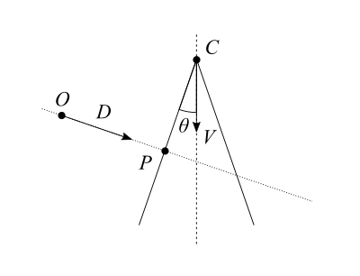
  1. We define a ray with its origin $O$ and its direction as a unit vector $\hat{D}$.
    Any point $X$ on the ray at a signed distance $t$ from the origin of the ray verifies: $\vec{X} = \vec{O} + t\vec{D}$.
    When $t$ is positive $X$ is in the direction of the ray, and when $t$ is negative $X$ is in the opposite direction.
  2. We define a cone with its tip $C$, its axis as a unit vector $\hat{V}$ in the direction of increasing radius, and $\theta$ the half angle between the axis and the surface.
    Any point $X$ on the cone verifies: $(\vec{X} – \vec{C}) \cdot \vec{V} = \lVert \vec{X} – \vec{C} \rVert \cos\theta$
  3. Finally we define $P$ the intersection or the ray and the cone, and which we are interested in finding.
$P$ verifies both equations, so we can write:

$$
\left\{
\begin{array}{l}
\vec{P}=\vec{O} + t\vec{D} \\
\frac{ \vec{P} – \vec{C} }{\lVert \vec{P} – \vec{C} \rVert} \vec{V} = \cos\theta
\end{array}
\right.
$$

We can multiply the second equation by itself to work with it, then reorder things a bit.

$$
\left\{
\begin{array}{l}
\vec{P}=\vec{O} + t\vec{D} \\
\frac{ ((\vec{P} – \vec{C}) \cdot \vec{V})^2 }{ (\vec{P} – \vec{C}) \cdot (\vec{P} – \vec{C}) } = \cos^2\theta
\end{array}
\right.
$$

$$
\left\{
\begin{array}{l}
\vec{P}=\vec{O} + t\vec{D} \\
((\vec{P} – \vec{C}) \cdot \vec{V})^2 – (\vec{P} – \vec{C}) \cdot (\vec{P} – \vec{C}) \cos^2\theta = 0
\end{array}
\right.
$$

Remember the mouthful earlier about $\hat{V}$ being in the direction of increasing radius? By elevating $\cos\theta$ to square, we’re making negative values of $\cos$ positive: values of $\theta$ beyond 90° become indistinguishable from values below 90°. This has the side effect of turning it into the equation of not one, but two cones sharing the same axis, tip and angle, but in opposite directions. We’ll fix that later.

We replace $\vec{P}$ with $\vec{O} + t\vec{D}$ and work the equation until we get a good old quadratic function that we can solve.

$$
\require{cancel}
((\vec{O} + t\vec{D} – \vec{C})\cdot\vec{V})^2 – (\vec{O} + t\vec{D} – \vec{C}) \cdot (\vec{O} + t\vec{D} – \vec{C}) \cos^2\theta = 0
$$

$$
((t\vec{D} + \vec{CO})\cdot\vec{V})^2 – (t\vec{D} + \vec{CO}) \cdot (t\vec{D} + \vec{CO}) \cos^2\theta = 0
$$

$$
(t\vec{D}\cdot\vec{V} + \vec{CO}\cdot\vec{V})^2 – (t^2\cancel{\vec{D}\cdot\vec{D}} + 2t\vec{D}\cdot\vec{CO} + \vec{CO}\cdot\vec{CO}) \cos^2\theta = 0
$$

$$
(t^2(\vec{D}\cdot\vec{V})^2 + 2t(\vec{D}\cdot\vec{V})(\vec{CO}\cdot\vec{V}) + (\vec{CO}\cdot\vec{V})^2) – (t^2 + 2t\vec{D}\cdot\vec{CO} + \vec{CO}\cdot\vec{CO}) \cos^2\theta = 0
$$

$$
t^2(\vec{D}\cdot\vec{V})^2
+ 2t(\vec{D}\cdot\vec{V})(\vec{CO}\cdot\vec{V})
+ (\vec{CO}\cdot\vec{V})^2
– t^2\cos^2\theta
– 2t\vec{D}\cdot\vec{CO}\cos^2\theta
– \vec{CO}\cdot\vec{CO}\cos^2\theta
= 0
$$

Reorder a bit:

$$
t^2((\vec{D}\cdot\vec{V})^2 – \cos^2\theta)
+ 2t((\vec{D}\cdot\vec{V})(\vec{CO}\cdot\vec{V}) – \vec{D}\cdot\vec{CO}\cos^2\theta)
+ (\vec{CO}\cdot\vec{V})^2 – \vec{CO}\cdot\vec{CO}\cos^2\theta
= 0
$$

There we go, we have our $at^2 + bt + c = 0$ equation, with:

$$
\left\{
\begin{array}{l}
a = (\vec{D}\cdot\vec{V})^2 – \cos^2\theta \\
b = 2\Big((\vec{D}\cdot\vec{V})(\vec{CO}\cdot\vec{V}) – \vec{D}\cdot\vec{CO}\cos^2\theta\Big) \\
c = (\vec{CO}\cdot\vec{V})^2 – \vec{CO}\cdot\vec{CO}\cos^2\theta
\end{array}
\right.
$$

From there, you know the drill: calculate the determinant $\Delta = b^2 – 4ac$ then depending on its value:

  • If $\Delta < 0$, the ray is not intersecting the cone.
  • If $\Delta = 0$, the ray is intersecting the cone once at $t = \frac{-b}{2a}$.
  • If $\Delta > 0$, the ray is intersecting the cone twice, at $t_1 = \frac{-b – \sqrt{\Delta}}{2a}$ and $t_2 = \frac{-b + \sqrt{\Delta}}{2a}$.

But wait! We don’t have one cone but two, so we have to reject solutions that intersect with the shadow cone. $P$ must still verify $\frac{ \vec{P} – \vec{C} }{\lVert \vec{P} – \vec{C} \rVert} \vec{V} = \cos\theta$, or simply, if $\theta < 90°$: $(\vec{P} – \vec{C})\cdot\vec{V} > 0$.

Note that there is also the corner case of the ray tangent to the cone and having an infinity of solutions to consider. I’ve completely swept it under the rug since it doesn’t matter in the context I was, but if it does to you, you’ve been warned about it. Also remember to check the sign of $t$ to know whether $P$ is in the direction of the ray. You may need to determine which of $t_1$ or $t_2$ you want to use, which depends on your use case. For example is your ray origin inside or outside of the cone?


Now for a little sanity test, let’s consider the corner case $C=O$, where the ray origin is the tip of the cone (thanks Rubix for the suggestion!). We have $b=0$ and $c=0$ thus $\Delta=0$ and $t=\frac{-b}{2a}=0$ which is the expected result.

I also tried the cases $\theta=0$ and $\theta=\pi/2$, but expanding $\Delta$ proved too tedious to proceed to the end. So this is left as an exercise, as they say. :)


Finally, to demonstrate that the result is indeed correct, here is a glorious ray traced cone scene on ShaderToy:

I hope this can prove useful to others too.

Oh, and Happy New Year by the way!

The Chemical Brothers: “Wide Open”

Earlier this year at Tokyo Demo Fest 2016, we were honored with the presence of Solid Angle‘s founder, Marcos Fajardo, who did a long presentation of the Arnold renderer. Various examples of productions that involved Arnold were included, like captures from Iron Man or Elysium, but between those blockbusters one production in particular held my attention.

It was a long shot of a dancer turning limb after limb into a lattice body while performing. That film is in fact the music video of the song “Wide Open”, by the Chemical Brothers, and directed by Dom&Nic. It is a brilliant piece of technical and artistic work, that I can only recommend to watch.

Some of the details of the creation are shared in an article by the excellent fxguide, as well as in this interview for Solid Angle, like for example how they dealt with the challenges posed by a single long shot under varying natural light. Finally, there is this behind the scenes video from the studio, The Mill:

Metal materials study

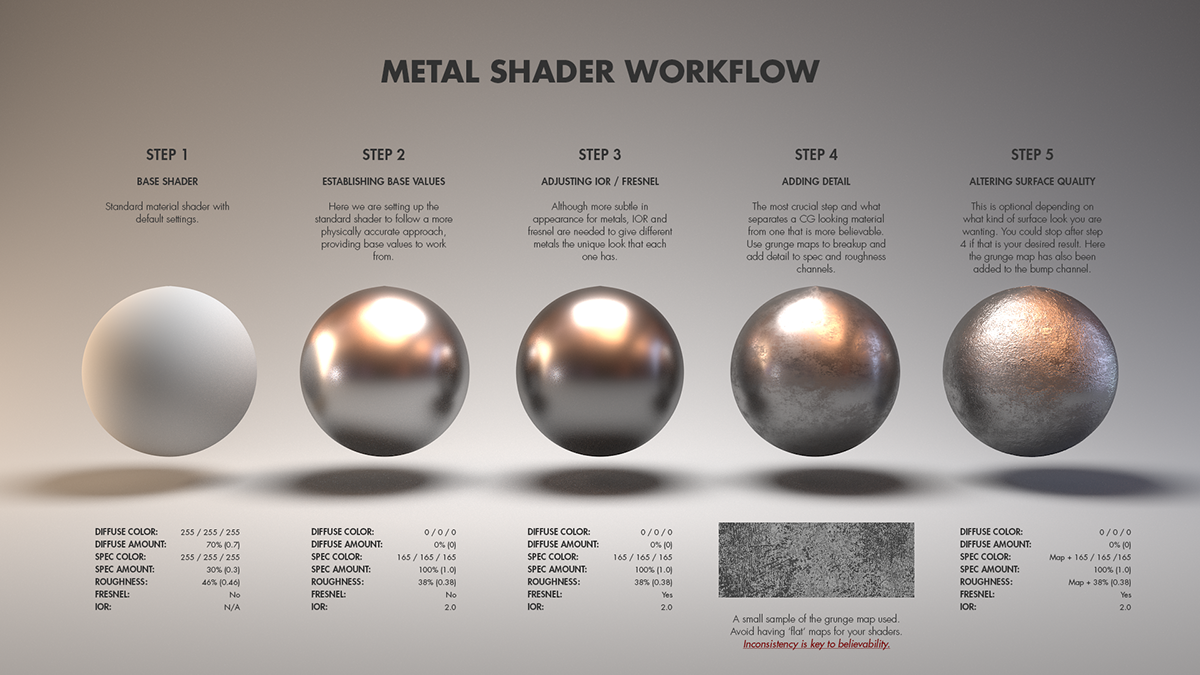
Texture artist Jarrod Hasenjager posted a page of various metal materials study: aluminum, brass, bronze, chrome, copper, gold, iron, lead and steel, and rusted steel and iron. According to the description, the renders are done in Houdini, and the look is driven by artistic taste and personal experience rather than from physical values.

Coordinate mapping between sphere, disc and square

This paper, published by Martin Lambers in the Journal of Computer Graphics Techniques, compares different mappings between sphere and disc, and between disc and square. It is worth noting that the source code is available on the publication page.

Mappings between Sphere, Disc, and Square.

Abstract:
A variety of mappings between a sphere and a disc and between a disc and a square, as well as combinations of both, are used in computer graphics applications, resulting in mappings between spheres and squares. Many options exist for each type of mapping; to pick the right methods for a given application requires knowledge about the nature and magnitude of mapping distortions.

This paper provides an overview of forward and inverse mappings between a unit sphere, a unit disc, and a unit square. Quality measurements relevant for computer graphics applications are derived from tools used in the field of map projection, and a comparative analysis of the mapping methods is given.

Series of articles on noise generation

I discovered last year these tutorials by Jasper Flick on how to make and use noise in Unity, and a couple of terrain and particle use examples. They present the difference between value noise and gradient noise, how Perlin noise and simplex noise work, and among others how to use curl noise to control the flow of particles.

The order information is presented is well thought, although the intention might not be clear at first. Don’t let the beginner’s tutorial tone (“You’ll learn to: create and fill a texture;”, etc.) turn you away, as the series do a great job at detailing the concepts and algorithms in a simple manner yet without cutting corners like so many articles on the topic do (when they’re not blatantly wrong and go ahead calling a blurred noise “Perlin noise”). I thought I had a pretty good grasp of gradient noise already, but reading it gave me an even better understanding.

Pushing particles around with Simplex curl noise.

While at it, other resources on the topic include Ken Perlin’s GDC 1999 talk and his two pages paper Improving noise explaining why use a 5th order polynomial for interpolation (a function I’ve sometimes seen called “smootherStep”).