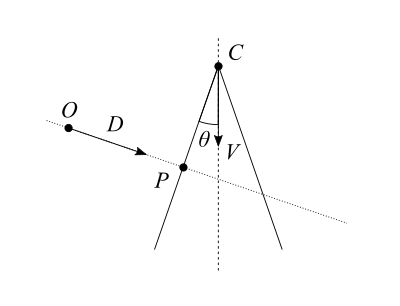
I previously showed the derivation of how to determine the intersection of a plane and a cone. At the time I had to solve that equation, so after doing so I decided to publish it for anyone to use. Given the positive feedback, it seems this was useful, so I might as well continue with a few more.
Here is probably the most basic intersection: a ray and a plane. Solving it is straightforward, which I hope can be seen below. Like last time, I am using vector notation.
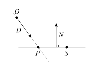
- We define a ray with its origin $O$ and its direction as a unit vector $\hat{D}$.
Any point $X$ on the ray at a signed distance $t$ from the origin of the ray verifies: $\vec{X} = \vec{O} + t\vec{D}$.
When $t$ is positive $X$ is in the direction of the ray, and when $t$ is negative $X$ is in the opposite direction. - We define a plane with a point $S$ on that plane and the normal unit vector $\hat{N}$, perpendicular to the plane.
The distance between any point $X$ and the plane is $d = \lvert (\vec{X} – \vec{S}) \cdot \vec{N} \rvert$. If this equality is not obvious for you, you can think of it as the distance between $X$ and $S$ along the $\vec{N}$ direction. When $d=0$, it means $X$ is on the plane itself. - We define $P$ the intersection or the ray and the plane, and which we are interested in finding.
Since $P$ is both on the ray and on the plane, we can write: $$ \left\{ \begin{array}{l} \vec{P}=\vec{O} + t\vec{D} \\ \lvert (\vec{P} – \vec{S}) \cdot \vec{N} \rvert = 0 \end{array} \right. $$ Because the distance $d$ from the plane is $0$, the absolute value is irrelevant here. We can just write: $$ \left\{ \begin{array}{l} \vec{P}=\vec{O} + t\vec{D} \\
(\vec{P} – \vec{S}) \cdot \vec{N} = 0 \end{array} \right. $$ All we have to do is replace $P$ with $\vec{O} + t\vec{D}$ in the second equation, and reorder the terms to get $t$ on one side.
$$ (\vec{O} + t\vec{D} – \vec{S}) \cdot \vec{N} = 0 $$ $$ \vec{O} \cdot \vec{N} + t\vec{D} \cdot \vec{N} – \vec{S} \cdot \vec{N} = 0 $$ $$ t\vec{D} \cdot \vec{N} = \vec{S} \cdot \vec{N} – \vec{O} \cdot \vec{N} $$ $$ t = \frac{(\vec{S} – \vec{O}) \cdot \vec{N}}{ \vec{D} \cdot \vec{N} } $$
A question to ask ourselves is: what about the division by $0$? Looking at the diagram, we can see that $\vec{D} \cdot \vec{N} = 0$ means the ray is parallel to the plane, and there is no solution unless $O$ is already on the plane. Otherwise, the ray intersects the plane for the value of $t$ written above. That’s it, we’re done.
Note: There are several, equivalent, ways of representing a plane. If your plane is not defined by a point $S$ and a normal vector $\hat{N}$, but rather with a distance to the origin $s$ and a normal vector $\hat{N}$, you can notice that $s = \vec{S} \cdot \vec{N}$ and simplify the result above, which becomes: $$ t = \frac{s – \vec{O} \cdot \vec{N}}{ \vec{D} \cdot \vec{N} } $$
Signed distance to a plane
For the sake of simplicity, in the above we defined the distance to the plane as an absolute value. It is possible however to define it as a signed value: $d = (\vec{X} – \vec{S}) \cdot \vec{N}$. In this case $d>0$ means $X$ is somewhere on the side of the plane pointed by $\vec{N}$, while $d<0$ means $X$ is on the opposite side of the plane.
Distances that can be negative are called signed distances, and they are a foundation of Signed Distance Fields (SDF).